Department of Physics and Astronomy, California State University Long Beach
Section
Introduction: Steel is one of the most used material industrially. Amounting to (put some stats here).
One concern with working with steel is rust. Many methods are used in order to negate the effects of corrosions (coating, polishing). However, it remains to be a costly issue for steel infrastructure (place some more stats here).
With climate change, the oceans are getting warmer and natural disasters such as hurricanes continue to intensify.
Talk about some theory:
Corrosion rate has a direct relationship to temperature. Increasing temperature of a solution will decrease the critical potential for corrosion to occur. This could be explained briefly with kinetic energy. The increased kinetic energy increases the reaction rates as well as the amount of chemical energy for a given reaction to occur.
Fe -> Fe2+ + 2e-
Cathodic half-cell reaction
O2 + 2H2O + 4e- -> 4OH-
Similarly, chloride acts as a catalysis for the oxidation reaction. Anions will assist in the electron transfer between the iron and oxygen.
Corrosion rate of carbon steel in seawater is 15 mpy in the first year then decreases to 5 mpy after 1000 days. Cite (E. McCafferty)
Experiment:
Sample Preparation
Samples are created from a commercially available 20 gauss steel sheet with dimensions 150 mm x 450 mm x 1.5 mm. The sheet metal is then cut into small sample sized squares using aviation snips.
A 3.5% saline solution is created for each sample using regular table salt. Corrosion is directly correlated to the logarithm of the chloride concentration of a solution (cite Leckie). All samples were submerged for 5 hours, let out to air dry, then again placed in another 5 hour bath.
We varied the temperature of the saline solution: 4 degrees Fridge C, 20 degrees C room temperature, 40 degrees C insulated bath and 60 degrees C heat pads.
Once samples are ready, they are prepared on a sample disk for measurement under the Park AFM. Double sided tape is required to adhere the corroded sheets onto the disk. The sample was mounted onto the sample stage within the Park AFM following the standard operating procedures.
Note: Data was taken on the first day for a control sample and the 20 degree sample. The scans showed a change in height for the sample varying around 800 nm. Given the limits of the cantilever, the higher temperature samples might cause damage to the AFM. The solution was to polish the steel using sanding paper. On the second day, control samples were measured for a polished sample. The topography was smooth compared to the original scans from the first day.
Day 3 of the experiment, the polishing technique was refined by using progressively higher grit sandpaper. The samples were then prepared as mentioned earlier.
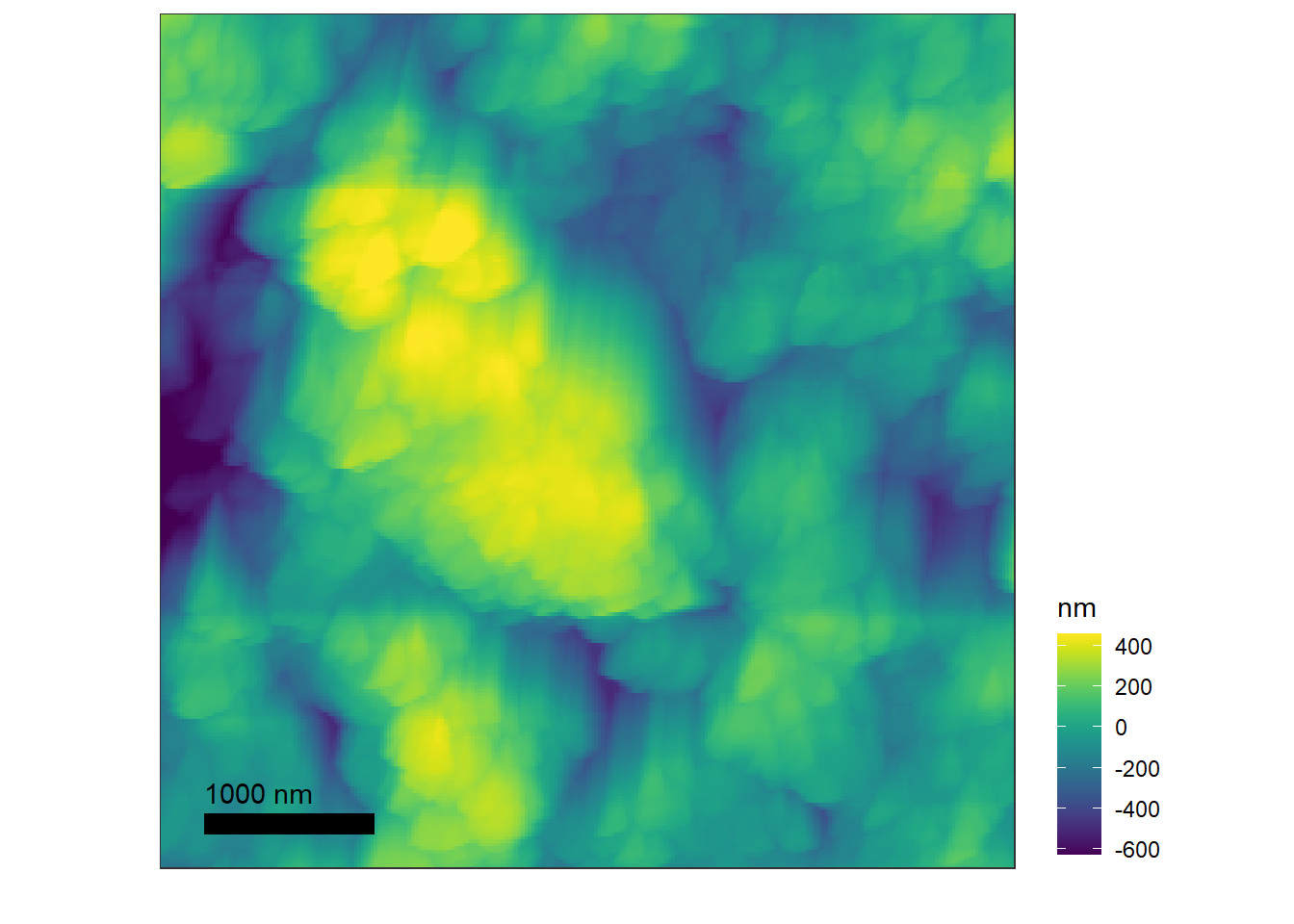
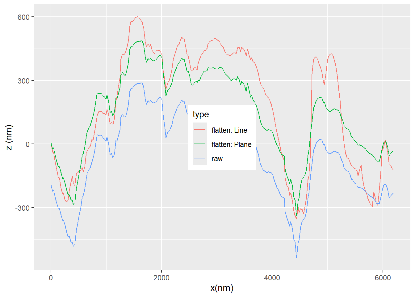
#Use the line by line flatten method to create flattened imageafmDataFlatLine =AFM.flatten(d, method="lineByLine")#Create a few line profiles of our flake across it's widthd1 =AFM.lineProfile(afmDataFlatLine, 46 , 254 , 219 , 10 ,unitPixels = T) -> bd11 =AFM.linePlot(b, dataOnly = T)d11$z = d11$z -354d11$type ="flatten: Line"
In [5]:
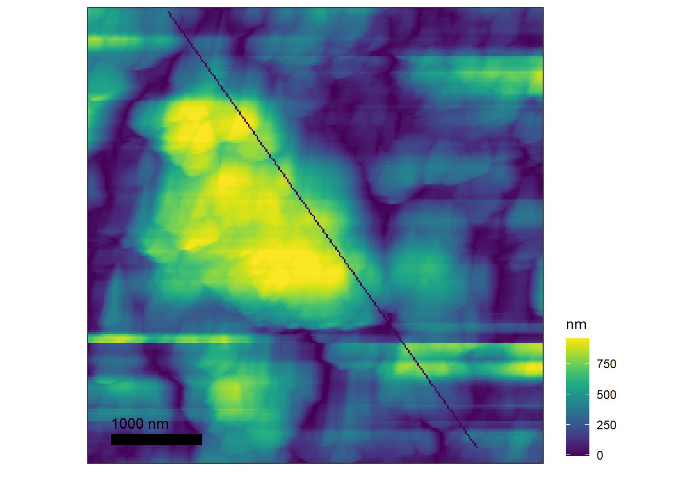
#Plot image with linesplot(b, graphType =2, addLines = T)
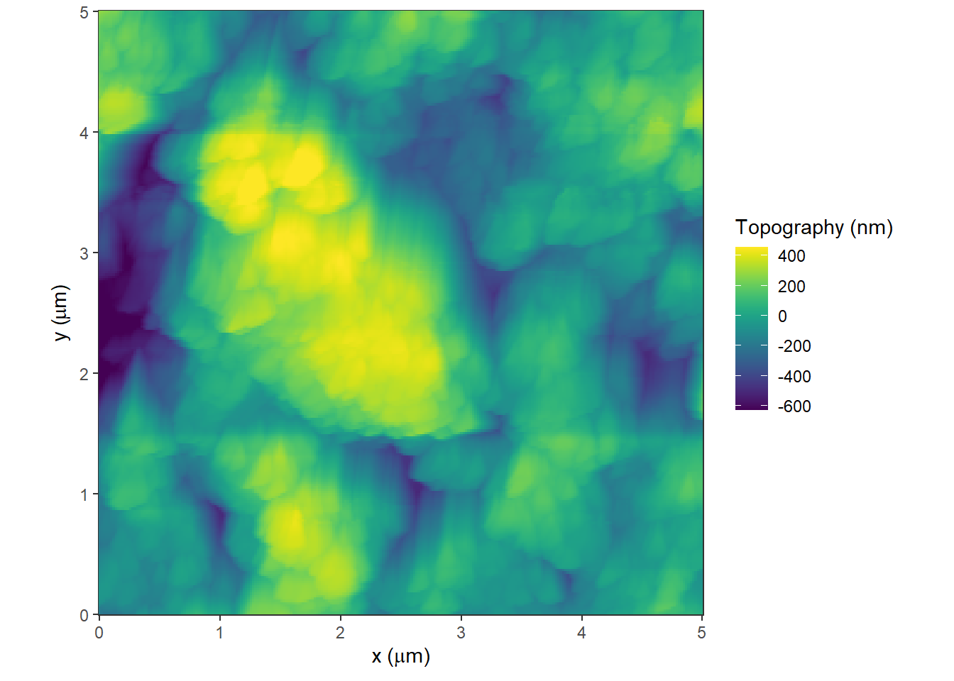
Graphing: Topography
Image of the refigerated sample flattened using the line by line technique.